Simulation is the consideration of all possible outcomes. We will use Python programming to implement petroleum simulations.
This tutorial on simulations consists of five sample programs run on PyCharm Community using the Python programming language. The first four programs run independently. The last program requires the previous three programs to run. All programs can be copy and pasted from this website to the PyCharm application. They all have been tested. The first program is BubbleSort which sorts a list of numbers from smallest to largest. The second program is UniformDistribution, the third program in TriangularDistribution, and the fourth program is GeneralDistribution. The fifth program is STOOIP which calculates the standard barrels of oil in a reservoir. It requires Distribution programs two, three, and four. These are sample programs that require modification for you particular needs. If you are new to Python programming I suggest the Amazon book Introduction to Engineering Python by Steve Larsen.(There is currently a workaround if the plot does not display in Linux Mint. You may see the error message UserWarning: Matplotlib is currently using agg. You must install two packages: Matplotlib and PyQt5).
Simulation is used in the evaluation of oil fields. When considering development of an oil field there are unknowns which must be approximated. Many times we can make approximations based on adjacent oil fields. These include the thickness of the sand layer containing the oil. The porosity of the sand layer, and the degree of oil saturation between the sand grains. There are two basic methods for making approximations. An engineer with experience may make an estimated single number guess for each value of the equation for oil production. It is probably more accurate to use a range of values for each parameter in the equation. This is where simulation comes in. Weighted numbers are used in calculations to approximate the final solution. Simulation considers all possible outcomes. There are three simulation distributions we will look at: Uniform, Triangular, and General. All require computer programming to solve. Python is an ideally suited computer program. It is relatively simple to learn. We will provide Python programs for solving the STOOIP equation below using Uniform, Triangular, and General Distributions.
We will use the following equation from petroleum engineering as an example of how to use simulation techniques.
To calculate volume of stock tank original oil in place (STOOIP) in barrels from volume measured in acre-feet, use the following formula:
STOOIP = 7758 x A x h x Porosity x (1 - Sw) / Bo
where:
There are three basic kinds of simulation distributions: uniform distributions, triangular distributions, and general distributions. A uniform distribution consists of a minimum and maximum value for approximation of a value in an equation. A triangular distribution consists of a minimum, maximum, and most likely intermediate value for approximation of a value in an equation. The general distribution covers all other cases, where there are many approximate values. For more information read Decision Analysis for Petroleum Exploration by Paul D. Newendorp, 1996.
The first parameter we will look at in the STOOIP equation is h or thickness of reservoir pay in feet. There are 20 wells in the surrounding area from which we can obtain values of sand thickness. We can use these 20 values to create a general distribution of thickness for the STOOIP equation. Once we have a program for the general distribution graph, we can use random values to evaluate the STOOIP equation. Many random values help us consider all possible outcomes from the general distribution. We will evaluate the STOOIP equation at 500 random values. (We could use 1000, or 1500 random values.) The 500 values of h will be stored in a Python list.
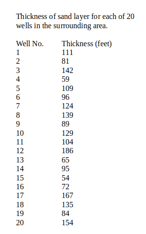
Thickness of sand layer for each of 20 wells sorted from smallest to largest (Use a Python bubble sort program.)
[54, 59, 65, 72, 81, 84, 89, 95, 96, 104, 109, 111, 124, 129, 135, 139, 142, 154, 167, 186]
Use the sorted values to find frequency of thicknesses in each range of thickness. See Column 1 and Column 2 in the chart below. Calculate the Cumulative Relative Frequency as shown in Column 3 and Column 4.
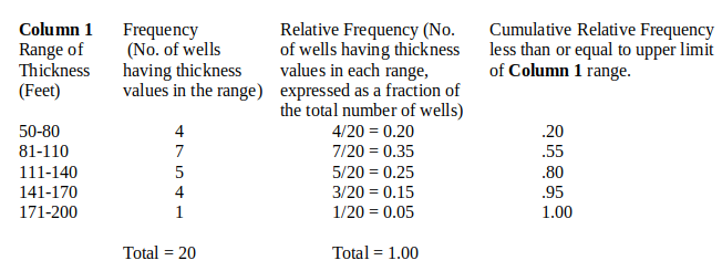
From the above data we create 6 sets of X-CF (Height-Cumulative Frequency) coordinates for the General Distribution.
X = [50,80,110,140,170,200]
CF = [0, .2, .55, .8, .95, 1]
We can create a graph of X vs CF, with X (Height) on the horizontal axis, and with CF (Cumulative Frequency) on the vertical axis. Given a random value for CF we can obtain a value for X (Height). We repeat this calculation 500 times. The list of 500 values is stored in a Python list called samplesX[]. We will insert each samplesX[] value to solve STOOIP[] equation 500 times.
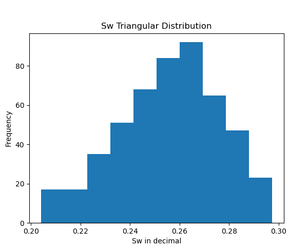
Next we will evaluate Sw in the STOOIP equation using the Triangular Distribution. Sw best guesses consist of a minimum value of 0.2, a maximum value of 0.3, and a most likely value of 0.27. Given a random value for CF we can obtain a value for Sw. We repeat this calculation 500 times The list of 500 values is stored in a Python list called samplesSw[]. We will insert each samplesSw[] value to solve STOOIP[] equation 500 times. Continue reading to see how Uniform Distributions can be used in the STOOIP equation.
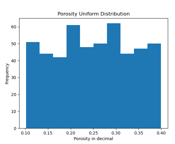
Next we will evaluate Porosity in the STOOIP equation using the Uniform Distribution. Porosity best guesses consist of a minimum value of 0.1, and a maximum value of 0.4. Given a random value for CF we can obtain a value for Porosity. We repeat this calculation 500 times The list of 500 values is stored in a Python list called samplesPorosity[]. We will insert each samplesPorosity[] value to solve STOOIP[] equation 500 times.
i = 1
while i < 499 : #Number of passes one less than in Distributions
STOOIP = 7758 * A * h[i] * Porosity[i] * (1 - Sw[i]) / Bo
samplesSTOOIP.append(STOOIP)
i = i + 1
The code snippet above provides us with a list of 500 values in samplesSTOOIP[]. We will now sort the values into a histogram to get the most likely value of STOOIP. This is simply done with the histogram() library plot in Python. We are done.
We start with the bubble sort program which sorts numbers from smallest to largest. At the top of the program a function is defined called the swap function. It will be called later. Next is the list to be sorted. Notice there are 20 items in the list, and the number 20 is typed in twice. In the center of the program we call the function. Finally the sorted list is printed.
#BubbleSort - Smallest to Largest

    #Functions have to be listed at top

    def myswap(a,b,alist):   #Swap function

       temp = alist[a]

       alist[a] = alist[b]

       alist[b] = temp

       return alist


    # List to be sorted

    mylist = [111,81,142,59,109,96,124,139,89,129,104,186,65,95,54,72,167,135,84,154]

    i = 0

    j = 0

    while i < 20:   # There are 20 items in list

       j = i + 1

       while j < 20:

          if mylist[i] > mylist[j]:

             mylist = myswap(i,j,mylist)

                   j = j + 1

             i = i + 1

    print(mylist)


    #Output [54, 59, 65, 72, 81, 84, 89, 95, 96, 104, 109, 111, 124, 129, 135, 139, 142, 154, 167, 186]
The next program to be shown is the Python General Distribution program. We use import random to provide for the random number generator later on. We input the number of sets, and the X-CF coordinates themselves. We initialize the list samplesX=[]. We begin our first while loop which repeats the random number generator and inner loop 500 times. We then solve the equation for the inner loop using the sets of coordinates; one set of coordinates at a time. The cumulative frequency is set equal to a random number. We then solve an equation for a straight line. Where X (height of sand thickness) corresponds to the cumulative frequency. The inner loop is repeated 500 times and the heights are added to a list of calculated heights, samplesX[]. See Decision Analysis for Petroleum Exploration by Paul D. Newendorp 1996. Following this are print statements to evaluate the program. Finally, a Python histogram is plotted to quickly evaluate the results.
      #Program named GeneralDistribution

      import random

      #sets of X-CF coordinates for GeneralDistribution

      sets = 6

      X = [50,80,110,140,170,200]

      CF = [0,.2,.55,.8,.95,1]


      samplesX = []

      i=1

      while i < 500:

         n = 0

         samCF = random.random()

         while n <= (sets-1) :

            if samCF <= CF[n+1] :

               samX = X[n] + (samCF - CF[n]) * (X[n+1] - X[n]) / (CF[n+1] - CF[n])

               samplesX.append(samX)

               break

            else :

               n = n+1

               continue

                     i = i+1

      #print('samCF=',samCF)

      #print('samX=', samX)

      #print('samplesX=', samplesX)


      import matplotlib.pyplot as plt

      plt.hist(samplesX)

      plt.title("Thickness General Distribution")

      plt.xlabel("Thickness-Feet")

      plt.ylabel("Frequency")

      plt.show()

The next program to be shown is the Python Triangular Distribution program. First we use import random to provide for the random number generator later on in the program. Next we enter the minimum, maximum, and most likely values for Sw. We then initialize samplesX=[]. We begin a while loop which repeats the random number generator 500 times. A random number is assigned to a cumulative frequency, and a value of Sw calculated. See Decision Analysis for Petroleum Exploration by Paul D. Newendorp 1996. The Sw value is appended onto the samplesSw[] list. Following this are print statements to evaluate the program. Finally, a Python histogram is plotted to quickly evaluate the results.
  #Program named TriangularDistribution

  import random

  #Min, Max, and Most Likely values for TriangularDistribution

  XMIN = .2

  XMODE =.27

  XMAX = .3


  samplesX = []

  i = 1

  while i < 500 :

     samCF = random.random()

     if samCF <= (XMODE - XMIN)/(XMAX - XMIN):

        samX = XMIN + (XMAX - XMIN)*(samCF*(XMODE - XMIN)/(XMAX - XMIN))**.5

             else:

                samX = XMIN + (XMAX - XMIN)*(1 - ((1 - samCF)*(1 - (XMODE - XMIN)/(XMAX - XMIN)))**.5)

             samplesX.append(samX)

             samplesSw = samplesX

             i = i + 1

  #print('samCF=',samCF)

  #print('samX',samX)

  #print('samplesX= ',samplesX)


  import matplotlib.pyplot as plt

  plt.hist(samplesSw)

  plt.title('Sw Triangular Distribution')

  plt.xlabel('Sw in decimal')

  plt.ylabel('Frequency')

  plt.show()
The next program to be shown is the Python Uniform Distribution program. First we use import random to provide for the random number generator later on in the program. Next we enter the minimum, and maximum values for Porosity. We then initialize samplesX=[]. We begin a while loop which repeats the random number generator 500 times. A random number is assigned to a cumulative frequency, and a value of Porosity calculated. See Decision Analysis for Petroleum Exploration by Paul D. Newendorp 1996. The Porosity value is appended onto the samplesPorosity[] list. Finally, a Python histogram plot to quickly evaluate the results.
  #Program named UniformDistribution

  import random

  #Min, Max for UniformDistribution

  XMIN = .10

  XMAX = .40


  samplesX = []

  i=1

  while i < 500:

     samCF = random.random()

     samX = XMIN + samCF*(XMAX - XMIN)

     samplesX.append(samX)

     samplesPorosity = samplesX

     i=i+1


  import matplotlib.pyplot as plt

  plt.hist(samplesPorosity)

  plt.title("Porosity Uniform Distribution")

  plt.xlabel('Porosity in decimal')

  plt.ylabel('Frequency')

  plt.show()
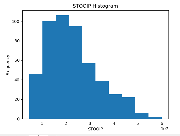
The final program calculates the most probable value of STOOIP. Note: When running the final program, it is linked to the three previous Distribution programs, and the plot for each program will be displayed. You must close each plot pop-up to get to the final STOOIP Plot. First we initialize samplesSTOOIP as a list. Next import the variable samplesPorosity from the UniformDistribution program. Import samplesSw from the TriangularDistribution program. Import samplesX from the GeneralDistribution program. Loop from 1 to 499. Each pass of the loop calculates a weighted value of STOOIP. We then plot a histogram of the STOOIP values to find the most likely value of STOOIP. That completes the task of finding the most likely value of STOOIP.
#Simulation solution to STOOIP equation

  samplesSTOOIP = []

  import UniformDistribution

  Porosity = UniformDistribution.samplesPorosity

  import TriangularDistribution

  Sw = TriangularDistribution.samplesSw

  import GeneralDistribution

  h = GeneralDistribution.samplesX

  A = 160

  Bo = 1.05


  i = 1

  while i < 499 : #Number of passes one less than in Distributions

     STOOIP = 7758 * A * h[i] * Porosity[i] * (1 - Sw[i]) / Bo

     samplesSTOOIP.append(STOOIP)

     i = i + 1

  import matplotlib.pyplot as plt

  plt.hist(samplesSTOOIP)

  plt.title("STOOIP Histogram")

  plt.xlabel('STOOIP')

  plt.ylabel('Frequency')

  plt.show()
There are other factors to consider prior to drilling. The Recovery Factor is the percent of oil we recover from the reservoir. The likely-hood of drilling a dry hole, and the cost of development of a producing well. See Decision Analysis for Petroleum Exploration by Paul D. Newendorp 1996.