
The online GPU (Graphical Processing Unit) capabilities include processing Keras, and TensorFlow environments. Google's site is called Google Colaboratory and is available on Google Drive. On this page we will give a detailed analysis of a deep learning program. There are two other pages of the tutorial that describe how to install Colab, and how to run a simple program. These are introductory tutorials.The deep learning program we use in the tutorial is written in Python. You can follow my Python tutorial if you so desire. Keras is built in Python.
Note: I strongly suggest getting the PDF copy of Deep Learning With Python Develop Deep Learning Models on Theano and TensorFlow Using Keras by Jason Brownlee. It is thorough and easy to understand.
We ran a simple neural network with Keras using the pima-indians-diabetes dataset. The pima-indians-diabetes dataset is a standard data set to compare machine learning programs. It compares traits for a large group of individuals to see if the onset of diabetes can be predicted. Here we will use a neural network program to evaluate the data set.
1.1 Download the pima-indians-diabetes.csv dataset to your computer from https://networkrepository.com/pima-indians-diabetes.php .
2.1 Use the following code to evaluate the pima-indians-diabetes.csv dataset. Be sure to use the proper upload name for pima-indians-diabetes.csv.
# first neural network with keras tutorial

        from numpy import loadtxt

        from keras.models import Sequential

        from keras.layers import Dense

        # load the dataset

        dataset = loadtxt("pima-indians-diabetes.csv", delimiter=',')

        # split into input (X) and output (y) variables

        # 0-8 are dependent variables- 8th column not included

        X = dataset[:,0:8]

        # 8 column is independent variable

        y = dataset[:,8]

        # define the keras model

        model = Sequential()

        model.add(Dense(12, input_dim=8, activation='relu'))

        model.add(Dense(8, activation='relu'))

        model.add(Dense(1, activation='sigmoid'))

        # compile the keras model

        model.compile(loss='binary_crossentropy', optimizer='adam', metrics=['accuracy'])

        # fit the keras model on the dataset

        model.fit(X, y, epochs=150, batch_size=16)

        # evaluate the keras model

        # Use _, to get last item from iteration

        _, accuracy = model.evaluate(X, y)

        print('Accuracy: %.2f'% (accuracy*100))
2.2 Use the following code to upload pima-indians-diabetes.csv file.
from google.colab import files

        uploaded = files.upload()
3.1 Run the program. You should see about 100 lines of output scroll through the output window on the lower left. There should be no error messages.
4.1 We will now describe what happens in each line of the program. I strongly suggest getting the PDF copy of Deep Learning With Python Develop Deep Learning Models on Theano and TensorFlow Using Keras by Jason Brownlee. It is thorough and easy to understand.
4.2 First, use the NumPy library to load the dataset and use two classes from Keras library to define our model. The imports are listed below.
# first neural network with keras tutorial

        from numpy import loadtxt

        from keras.models import Sequential

        from keras.layers import Dense


        ...
4.3 We load the file directly using the NumPy function loadtxt(). Use the file name pima-indians-diabetes.csv. CSV stands for comma separated values. The database is a rectangular array of 8 columns of X values (labeled 0 to 7) and one column of y values (labeled column 8). The y values in column 8 are either a one or a zero. 1 for onset of diabetes, and 0 for no onset of diabetes. The notation dataset[:,0:8] and dataset[:,8] are called array slicing. (You can see more about slicing in the Python tutorial. Array and Slicing Arrays in Python)
...


          # load the dataset

          dataset = loadtxt("pima-indians-diabetes.csv", delimiter=',')

          # split into input (X) and output (y) variables

          # 0-8 are dependent variables- 8th column not included

          X = dataset[:,0:8]

          # 8 column is independent variable

          y = dataset[:,8]


          ...
The labels for each column of the dataset are listed below.
1. Number of times pregnant (Column 0)
2. Plasma glucose concentration (Column 1)
3. Diastolic blood pressure (Column 2)
4. Triceps skin fold thickness (Column3)
5. 2-Hour serum insulin (Column 4)
6. Body mass index (Column 5)
7. Diabetes pedigree function (Column 6)
8. Age in years (Column 7)
9. 0 or 1 for onset of diabetes in 5 years (Column 8)
Below are the first 5 rows of 768 rows of data. One row per person.
6,148,72,35,0,33.6,0.627,50,1
1,85,66,29,0,26.6,0.351,31,0
8,183,64,0,0,23.3,0.672,32,1
1,89,66,23,94,28.1,0.167,21,0
0,137,40,35,168,43.1,2.288,33,1
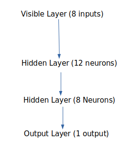
4.4 Next we define the Keras model. As a simplification, Keras is a set of functions used in evaluating neural networks models. Models in Keras are defined as a sequence of layers. The number of layers varies. It is a process of trial and error. We will use three layers. All layers are defined using the Dense class, for fully connected layers. The first layer has 12 neurons, has 8 input X values (from the database), and uses a relu activation function. The second layer has 8 neurons, and uses a relu activation function. The third layer has 1 neuron, and uses a sigmoid activation function. There is 1 neuron which is either 0 or 1 to signify diabetes. The sigmoid activation function is used to deliver a 0 or 1 with a .5 threshold to the y value.
...


        # define the keras model

        model = Sequential()

        model.add(Dense(12, input_dim=8, activation='relu'))

        model.add(Dense(8, activation='relu'))

        model.add(Dense(1, activation='sigmoid'))


        ...
4.5 Next we compile the Keras model. First we specify a loss function to evaluate the coefficient weights for the evaluating formulas. The loss function is called binary_crossentropy. Second we enter an optimization algorithm called adam. Third we define a accuracy metric for our results.
...


          # compile the keras model

          model.compile(loss='binary_crossentropy', optimizer='adam', metrics=['accuracy'])


          ...
4.6 We will now get coefficients for the model so that the model fits the data (X values), and predicts the (y value). This process involves iterating through the data set. Each iteration is called an epoch. The batch_size is the number of sets of X values we use before updating the weights. Remember that weights are coefficients for formulas. They are chosen by trial and error.
...


          # fit the keras model on the dataset

          model.fit(X, y, epochs=150, batch_size=16)


          ...
4.7 We will now evaluate the Keras model, and see what percent of the time it is accurate. The only tricky part here is the line above the print statement. The _, is used to set accuracy equal to the last value of the iterations from model.evaluate (X, y).
...


        # evaluate the keras model

        # Use _, to get last item from iteration

        _, accuracy = model.evaluate(X, y)

        print('Accuracy: %.2f'% (accuracy*100))
4.8 The model predicts y from the X’s input, about 77% of the time. In other words the model predicts diabetes correctly, 77% of the time.
